Long Short-term
Memory

R Packages

# install.packages("tsibble")
# install.packages("tsibbledata")

library(torch)
library(luz) # high-level interface for torch
library(tsibble)
library(tsibbledata)
torch_manual_seed(909)

Here is the complete R Code File

Python Data

import pandas as pd
vic_elec = pd.read_csv("https://raw.githubusercontent.com/inqs909/m408_s26/refs/heads/main/lectures/data/vic_elec.csv")

Sequential Data

Sequential Data
Long Short-term Memory
Predicting Electricity Demand

Sequential Data

Sequential data is data that is obtained in a series:

\[ X_{(0)}\rightarrow X_{(1)}\rightarrow X_{(2)}\rightarrow X_{(3)}\rightarrow \cdots\rightarrow X_{(J-1)}\rightarrow X_{(J)} \]

Stochastic Procceses

A stochastic process is a collection of random variables, that can be indexed by a parameters. Sequential data can be thought of as a stochastic process.

The generation of a variable \(X_{(j)}\) may or may not be dependent of the previous values.

Examples of Sequential Data

Documents and Books
Temperature
Stock Prices
Speech/Recordings
Handwriting

Long Short-term Memory

Sequential Data
Long Short-term Memory
Predicting Electricity Demand

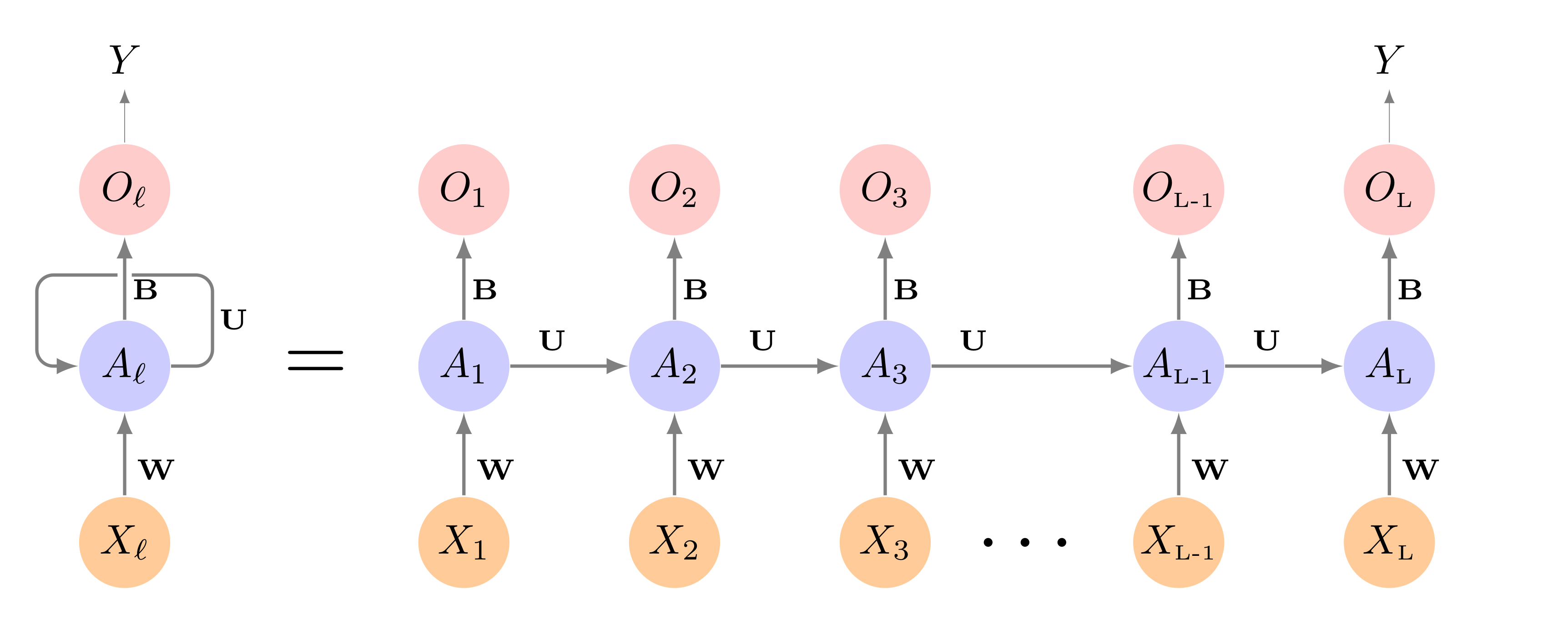
RNN

Recurrent Neural Networks are designed to analyze input data that is sequential data.

An RNN can accounts for the position of a data point in the sequence as well as the distance it has to other data points.

Using the data sequence, we can predict and outcome \(Y\).

RNN

Source: ISLR2

RNN Neuron

Problems with RNN

Recurrent Neural Networks suffer from exploding or disappearing gradient due the unfolding.

LSTM

The Long Short-Term Memory approach is used to conteract the issues with gradients by adding a “memory” structure to the nuerons.

This is done by incorporating 2 pathways, a long-term and short-term pathway.

LSTM Components

The creation of the 2 pathways are constructed using 3 “gates”:

Input Gate
Output Gate
Forget Gate

Additionally, LSTM uses sigmoid and hyperbolic tangent activation functions to see what values will be incorporated into the pathways.

LSTM Neuron

LSTM Architecture

Forget Gate

The forget gate decides what information is useful from the long-term memory, and what information should be forgotten. The function below states what percent of the long-term memory should be remembered. \[ f_t = \sigma\left(\boldsymbol W_f [h_{t-1}, x_t] + b_f\right) \]

\(W_f\) is the weighting matrix full of parameters
\(b_f\) is the bias term

Input Gate

The input gate controls how the long term memory should be modified based on both the short-term memory and the new input. The \(i_t\) function tells us what percent should be remembered, and \(j_t\) tells us what to remember. \[ i_t = \sigma\left(\boldsymbol W_i [h_{t-1}, x_t] + b_i\right) \]

\[ j_t = \tanh\left(\boldsymbol W_j [h_{t-1}, x_t] + b_j\right) \]

\(W_i\) and \(W_j\) is the weighting matrix full of parameters
\(b_i\) and \(b_j\) is the bias term

Long-term Memory

This is how the long-term memory is modified

\[ C_t = f_t \bigodot C_{t-1} + i_t \bigodot j_t \]

\(\bigodot\) is the element-wise multiplication of the vectors

Output Gate

The output gate tells us how is the short-term memory is updated. This is dony by figuring out what percent will be used from the new long-term memory.

\[ o_t = \sigma\left(\boldsymbol W_o [h_{t-1}, x_t] + b_o\right) \]

\(W_o\) is the weighting matrix full of parameters
\(b_o\) is the bias term

Short-term Memory

The short-term memory is costructed by combining the output gate and new long-term memory. \[ h_t = o_t\tanh\left(C_t\right) \]

This is also the new predicted value.

Predicting Electricity Demand

Sequential Data
Long Short-term Memory
Predicting Electricity Demand

Predicting Electricity Demand

We will use the vic_elec data set to be able to predict what the demand will be in a future time point.

Data Set

In order to fit a model with Torch, we need to provide a data set funcion that provides 2 values, a set of input and set of output. With Sequential data, values may be both outputs and inputs. We will use the dataset() to ensure that values can be used as both output and input.

RNN Neuron

Instead of the standard RNN Neuron, we will implement the Long Short-Term Memory Neuron.

# install.packages("torchdatasets")
# install.packages("feasts")

library(tidyverse)
library(torch)
library(luz) # high-level interface for torch

torch_manual_seed(909)
library(tsibble)
library(tsibbledata)
vic_ele

demand_dataset <- dataset(
  name = "demand_dataset",
  initialize = function(x,
                        n_timesteps,
                        n_forecast,
                        sample_frac = 1) {
    self$n_timesteps <- n_timesteps
    self$n_forecast <- n_forecast
    self$x <- torch_tensor((x - train_mean) / train_sd)

    n <- length(self$x) -
      self$n_timesteps - self$n_forecast + 1

    self$starts <- sort(sample.int(
      n = n,
      size = n * sample_frac
    ))
  },
  .getitem = function(i) {
    start <- self$starts[i]
    end <- start + self$n_timesteps - 1

    list(
      x = self$x[start:end],
      y = self$x[(end + 1):(end + self$n_forecast)]$
        squeeze(2)
    )
  },
  .length = function() {
    length(self$starts)
  }
)

demand_hourly <- vic_elec |> 
  index_by(Hour = floor_date(Time, "hour")) |> 
  summarise(
    Demand = sum(Demand))

demand_train <- demand_hourly |> 
  filter(year(Hour) == 2012) |> 
  as_tibble() |> 
  select(Demand) |> 
  as.matrix()

demand_valid <- demand_hourly |> 
  filter(year(Hour) == 2013) |> 
  as_tibble() |> 
  select(Demand) |> 
  as.matrix()

demand_test <- demand_hourly |> 
  filter(year(Hour) == 2014) |> 
  as_tibble() |> 
  select(Demand) |> 
  as.matrix()

train_mean <- mean(demand_train)
train_sd <- sd(demand_train)

n_timesteps <- 7 * 24
n_forecast <- 7 * 24

train_ds <- demand_dataset(
  demand_train,
  n_timesteps,
  n_forecast,
  sample_frac = 1
)
valid_ds <- demand_dataset(
  demand_valid,
  n_timesteps,
  n_forecast,
  sample_frac = 1
)
test_ds <- demand_dataset(
  demand_test,
  n_timesteps,
  n_forecast
)

batch_size <- 128
train_dl <- train_ds |> 
  dataloader(batch_size = batch_size, shuffle = TRUE)
valid_dl <- valid_ds |> 
  dataloader(batch_size = batch_size)
test_dl <- test_ds |> 
  dataloader(batch_size = length(test_ds))

Model

Model
Initialize
Forward

model <- nn_module(
  initialize = function(input_size,
                        hidden_size,
                        linear_size,
                        output_size,
                        dropout = 0.2,
                        num_layers = 1,
                        rec_dropout = 0) {
    self$num_layers <- num_layers

    self$rnn <- nn_lstm(
      input_size = input_size,
      hidden_size = hidden_size,
      num_layers = num_layers,
      dropout = rec_dropout,
      batch_first = TRUE
    )

    self$dropout <- nn_dropout(dropout)
    self$mlp <- nn_sequential(
      nn_linear(hidden_size, linear_size),
      nn_relu(),
      nn_dropout(dropout),
      nn_linear(linear_size, output_size)
    )
  },
  forward = function(x) {
    x <- self$rnn(x)[[2]][[1]][self$num_layers, , ] |> 
      self$mlp()
  }
)

  initialize = function(input_size,
                        hidden_size,
                        dropout = 0.2,
                        num_layers = 1,
                        rec_dropout = 0) {
    self$num_layers <- num_layers

    self$rnn <- nn_lstm(
      input_size = input_size,
      hidden_size = hidden_size,
      num_layers = num_layers,
      dropout = rec_dropout,
      batch_first = TRUE
    )

    self$dropout <- nn_dropout(dropout)
    self$output <- nn_linear(hidden_size, 1)
  }

  forward = function(x) {
    (x |> 
      self$rnn())[[1]][, dim(x)[2], ] |> 
      self$dropout() |> 
      self$output()
  }

Training

Setup
Train
Evaluate

input_size <- 1
hidden_size <- 32
linear_size <- 512
dropout <- 0.5
num_layers <- 2
rec_dropout <- 0.2

model <- model |> 
  setup(optimizer = optim_adam, loss = nn_mse_loss()) |> 
  set_hparams(
    input_size = input_size,
    hidden_size = hidden_size,
    linear_size = linear_size,
    output_size = n_forecast,
    num_layers = num_layers,
    rec_dropout = rec_dropout
  )

fitted <- model |> 
  fit(train_dl, epochs = 30, valid_data = valid_dl,
      verbose = TRUE)

plot(fitted)

evaluate(fitted, test_dl)

Predict and Visualize

demand_viz <- demand_hourly |> 
  filter(year(Hour) == 2014, month(Hour) == 12)

demand_viz_matrix <- demand_viz |> 
  as_tibble() |> 
  select(Demand) |> 
  as.matrix()

n_obs <- nrow(demand_viz_matrix)

viz_ds <- demand_dataset(
  demand_viz_matrix,
  n_timesteps,
  n_forecast
)
viz_dl <- viz_ds |> 
  dataloader(batch_size = length(viz_ds))

preds <- predict(fitted, viz_dl)
preds <- preds$to(device = "cpu") |> 
  as.matrix()

example_preds <- vector(mode = "list", length = 3)
example_indices <- c(1, 201, 401)

for (i in seq_along(example_indices)) {
  cur_obs <- example_indices[i]
  example_preds[[i]] <- c(
    rep(NA, n_timesteps + cur_obs - 1),
    preds[cur_obs, ],
    rep(
      NA,
      n_obs - cur_obs + 1 - n_timesteps - n_forecast
    )
  )
}

pred_ts <- demand_viz |> 
  select(Demand) |> 
  add_column(
    p1 = example_preds[[1]] * train_sd + train_mean,
    p2 = example_preds[[2]] * train_sd + train_mean,
    p3 = example_preds[[3]] * train_sd + train_mean) |> 
  pivot_longer(-Hour) |> 
  update_tsibble(key = name)

pred_ts |> 
    ggplot(aes(Hour, value, color = name)) +
      geom_line() +
  scale_colour_manual(
    values = c(
      "#08c5d1", "#00353f", "#ffbf66", "#d46f4d"
    )
  ) +
  theme_minimal() +
  theme(legend.position = "None")