Word Embeddings
All Models are Wrong, some are useful!
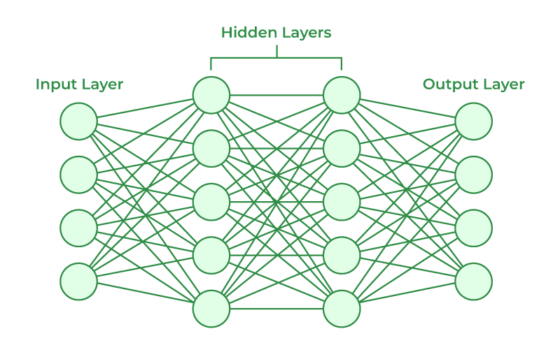
How do we input this into a neural network?
Youtube Video