Deep Learning

Neural Networks

Neural Networks
Stochastic Gradient Descent
R6
TensorFlow
Torch
R Code
Single Layer R Code
Multilayer R Code

Neural Networks

Neural networks are a type of machine learning algorithm that are designed to mimic the function of the human brain. They consist of interconnected nodes or “neurons” that process information and generate outputs based on the inputs they receive.

Uses

Neural networks are typically used for tasks such as image recognition, natural language processing, and prediction. They are capable of learning from data and improving their performance over time, which makes them well-suited for complex and dynamic problems.

Single Layer Neural Networks

A single layer neural networks can be formulated as linear function:

\[ f(X) = \beta_0 + \sum^K_{k=1}\beta_kh_k(X) \]

Where \(X\) is a vector of inputs of length \(p\) and \(K\) is the number of activations, \(\beta_j\) are the regression coefficients and

\[ h_k(X) = A_k = g(w_{k0} + \sum^p_{l1}w_{kl}X_{l}) \]

with \(g(\cdot)\) being a nonlinear function and \(w_{kl}\) are the weights.

Nonlinear (Activations) Function \(g(\cdot)\)

Sigmoidal: \(g(z) = \frac{e^z}{1+e^z}\)
ReLU (rectified linear unit): \(g(z) = (z)_+ = zI(z\geq0)\)

Single Layer Neural Network

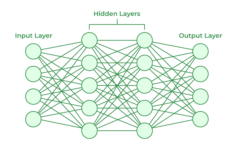
Multilayer Neural Network

Multilayer Neural Networks create multiple hidden layers where each layer feeds into each other which will create a final outcome.

Multilayer Neural Network

Hidden Layer 1

With \(p\) predictors of \(X\):

\[ h^{(1)}_k(X) = A^{(1)}_k = g\left\{w^{(1)}_{k0} + \sum^p_{j=1}w^{(1)}_{kj}X_{j}\right\} \] for \(k = 1, \cdots, K\) nodes.

Hidden Layer 2

\[ h^{(2)}_l(X) = A^{(2)}_l = g\left\{w^{(2)}_{l0} + \sum^K_{k=1}w^{(2)}_{lk}A^{(1)}_{k}\right\} \] for \(l = 1, \cdots, L\) nodes.

Hidden Layer 3 +

\[ h^{(3)}_m(X) = A^{(3)}_l = g\left\{w^{(3)}_{m0} + \sum^L_{l=1}w^{(3)}_{ml}A^{(2)}_{l}\right\} \] for \(m = 1, \cdots, M\) nodes.

Output Layer

\[ f_t(X) = \beta_{t0} + \sum^M_{m=1}\beta_{tm}h^{(3)}_m(X) \] for outcomes \(t = 1, \cdots, T\)

Stochastic Gradient Descent

Neural Networks
Stochastic Gradient Descent
R6
TensorFlow
Torch
R Code
Single Layer R Code
Multilayer R Code

Gradient Descent

This is an optimization algorithm used to identify the maximum or minimum of a functions.

Method

For a given \(F(\boldsymbol X)\), the minimum \(\boldsymbol X^\prime\) can be found by iterating the following formula:

\[ \boldsymbol X_{j+1} = \boldsymbol X_{j} - \gamma \nabla F(\boldsymbol X_j) \] where

\[ \boldsymbol X_j \rightarrow \boldsymbol X^\prime \]

\(\nabla F\): gradient
\(\gamma \in (0,1]\): is the step size

Stochastic Gradient Descent

Let:

\[ F(\boldsymbol X) = \sum^n_{i=1} f(y_i; \boldsymbol X) \]

Instead of minimizing \(F(\boldsymbol X)\) at each step, we minimize:

\[ F_\alpha(\boldsymbol X) = \sum_{i\in\alpha} f(y_i; \boldsymbol X) \] where \(\alpha\) indicates the data points randomly sampled to be used to compute the gradient.

R6

Neural Networks
Stochastic Gradient Descent
R6
TensorFlow
Torch
R Code
Single Layer R Code
Multilayer R Code

Object-Oriented Programming

Loosely speaking Object-Oriented Programming involves developing R objects with specialized attributes.

There are 3 main types of OOP: S3, R6, S4

xlm <- lm(mpg ~ wt, mtcars)
attributes(xlm)

#> $names
#>  [1] "coefficients"  "residuals"     "effects"       "rank"         
#>  [5] "fitted.values" "assign"        "qr"            "df.residual"  
#>  [9] "xlevels"       "call"          "terms"         "model"        
#> 
#> $class
#> [1] "lm"

sloop::s3_methods_generic("summary")

#> # A tibble: 37 × 4
#>    generic class                 visible source             
#>    <chr>   <chr>                 <lgl>   <chr>              
#>  1 summary aov                   TRUE    stats              
#>  2 summary aovlist               FALSE   registered S3method
#>  3 summary aspell                FALSE   registered S3method
#>  4 summary check_packages_in_dir FALSE   registered S3method
#>  5 summary connection            TRUE    base               
#>  6 summary data.frame            TRUE    base               
#>  7 summary Date                  TRUE    base               
#>  8 summary default               TRUE    base               
#>  9 summary ecdf                  FALSE   registered S3method
#> 10 summary factor                TRUE    base               
#> # ℹ 27 more rows

R6

R6 is slightly different, where the generic functions belong to the object instead.

This allows us to modify an R objects with different methodologies if needed.

This is also useful when interacting with objects outside of R’s environment.

`self`

self is a special container within R6 that contains all the items and functions within the object.

You must always use self when dealing with R6 objects.

TensorFlow

Neural Networks
Stochastic Gradient Descent
R6
TensorFlow
Torch
R Code
Single Layer R Code
Multilayer R Code

TensorFlow

Tensorflow is an open-source machine learning platform developed by Google. Tensorflow is capable of completing the following tasks:

Image Classification
Text Classification
Regression
Time-Series

Keras

Keras is the API that will talk to Tensorflow via different platforms.

More Information

TensorFlow for R

Torch

Neural Networks
Stochastic Gradient Descent
R6
TensorFlow
Torch
R Code
Single Layer R Code
Multilayer R Code

Torch

Torch is a scientific computing framework designed to support machine learning in CPU/GPU computing. Torch is capable of computing:

Matrix Operations
Linear Algebra
Neural Networks
Numerical Optimization
and so much more!

Torch

Torch can be accessed in both:

Pytorch
R Torch

R Torch

R Torch is capable of handling:

Image Recognition
Tabular Data
Time Series Forecasting
Audio Processing

More Information

R Code

Neural Networks
Stochastic Gradient Descent
R6
TensorFlow
Torch
R Code
Single Layer R Code
Multilayer R Code

Installation of Torch

install.packages("torch")
install.packages("luz")
install.packages("torchvision")
install.packages("torchdatasets")
install.packages("zeallot")

Torch Packages in R

# 
library(torch)
library(luz) # high-level interface for torch
library(torchvision) # for datasets and image transformation
library(torchdatasets) # for datasets we are going to use
library(zeallot)
torch_manual_seed(13)

ISLR Torch Lab

ISLR uses Tensorflow.

Use this instead: https://hastie.su.domains/ISLR2/Labs/Rmarkdown_Notebooks/Ch10-deeplearning-lab-torch.html

Single Layer R Code

Neural Networks
Stochastic Gradient Descent
R6
TensorFlow
Torch
R Code
Single Layer R Code
Multilayer R Code

Build a single-layer neural network that will predict body_mass_g with the remaining predictors except for year. The hidden layer will contain 50 nodes, and the activation functions will be ReLU.

library(tidyverse)
library(palmerpenguins)


penguins <- penguins |> drop_na() |> select(-year)
training <- penguins |> slice_sample(prop = .8)
testing <- penguins |> anti_join(training)

Xtraining <- training |> 
  model.matrix(body_mass_g ~ . - 1, data = _) |> 
  scale() |> 
  torch_tensor(dtype = torch_float())

Ytraining <- training |> 
  select(body_mass_g) |> 
  as.matrix() |> 
  torch_tensor(dtype = torch_float())

Xtesting <- testing |> 
  model.matrix(body_mass_g ~ . - 1, data = _) |> 
  scale() |> 
  torch_tensor(dtype = torch_float())

Ytesting <- testing |> 
  select(body_mass_g) |> 
  as.matrix() |> 
  torch_tensor(dtype = torch_float())

Model Description

Overall
Initialize
Forward

modnn <- nn_module(
  initialize = function(input_size) {
    self$hidden <- nn_linear(input_size, 50)
    self$activation <- nn_relu()
    self$dropout <- nn_dropout(0.4)
    self$output <- nn_linear(50, 1)
  },
  forward = function(x) {
    x |> 
      self$hidden() |>  
      self$activation() |>  
      self$dropout() |>  
      self$output()
  }
)

Creates the functions needed to describe the details of each network.

initialize = function(input_size) {
    self$hidden <- nn_linear(input_size, 50)
    self$activation <- nn_relu()
    self$dropout <- nn_dropout(0.4)
    self$output <- nn_linear(50, 1)
  }

Models the neural network.

forward = function(x) {
    x |> 
      self$hidden() |>  
      self$activation() |>  
      self$dropout() |>  
      self$output()
  }

Optimizer Set Up

modnn <- modnn |> 
  setup(
    loss = nn_mse_loss(), # Used for numerical counts
    optimizer = optim_rmsprop,
    metrics = list(luz_metric_mae())
  ) |>
  set_hparams(input_size = ncol(Xtraining))

Fit a Model

Fit
Plot

fitted <- modnn |> 
  fit(
    data = list(Xtraining, Ytraining),
    epochs = 100 # Can think as number of iterations
  )

Code

plot(fitted)

Testing Model

Prediction
MAE
Plot

npred <- predict(fitted, Xtesting)

mean(abs(as.matrix(Ytesting) - as.matrix(npred)))

#> [1] 422.8148

Code

plot(as.matrix(Ytesting), as.matrix(npred),
     xlab = "Truth",
     ylab = "Predicted")

Multilayer R Code

Neural Networks
Stochastic Gradient Descent
R6
TensorFlow
Torch
R Code
Single Layer R Code
Multilayer R Code

Penguins Data

Description
Prep
Training
Testing

Use the penguins data set to construct a 2-layer neural network to predict species with the other predictors, except for year. The 1st layer should have 10 nodes, the second layer should have 5 nodes, and use ReLU activations.

training <- penguins |> slice_sample(prop = .8)
testing <- penguins |> anti_join(training)

Xtraining <- training |> 
  model.matrix(species ~ . - 1, data = _) |> 
  scale()

Xtesting <- testing |> 
  model.matrix(species ~ . - 1, data = _) |> 
  scale()

Ytraining <- training |> 
  select(species) |> 
  as.matrix() |> 
  as.factor()

Ytesting <- testing |> 
  select(species) |> 
  as.matrix() |> 
  as.factor()

Model

Overall
Initialize
Forward

modelnn2 <- nn_module(
  initialize = function(input_size) {
    self$hidden1 <- nn_linear(in_features = input_size, 
                              out_features = 10)
    self$hidden2 <- nn_linear(in_features = 10, 
                              out_features = 5)
    self$output <- nn_linear(in_features = 5, 
                             out_features = 3)
    
    self$drop1 <- nn_dropout(p = 0.4)
    self$drop2 <- nn_dropout(p = 0.3)
    
    self$activation <- nn_relu()
  },
  forward = function(x) {
    x |>  
      self$hidden1() |>  
      self$activation() |>  
      self$drop1() |>  
      
      self$hidden2() |>  
      self$activation() |>  
      self$drop2() |>  
      
      self$output()
  }
)

  initialize = function(input_size) {
    self$hidden1 <- nn_linear(in_features = input_size, 
                              out_features = 10)
    self$hidden2 <- nn_linear(in_features = 10, 
                              out_features = 5)
    self$output <- nn_linear(in_features = 5, 
                             out_features = 3)
    
    self$drop1 <- nn_dropout(p = 0.4)
    self$drop2 <- nn_dropout(p = 0.3)
    
    self$activation <- nn_relu()
  }

forward = function(x) {
    x |>  
      self$hidden1() |>  
      self$activation() |>  
      self$drop1() |>  
      
      self$hidden2() |>  
      self$activation() |>  
      self$drop2() |>  
      
      self$output()
  }

Setup

modelnn2 <- modelnn2 |> 
  setup(loss = nn_cross_entropy_loss(),
        optimizer = optim_rmsprop, 
        metrics = list(luz_metric_accuracy())) |>
  set_hparams(input_size = ncol(Xtraining))

Model Fitting

Fit
Plot

fitted2 <- modelnn2 |> 
  fit(data = list(Xtraining, Ytraining), 
      epochs = 100)

plot(fitted2)

Testing

res <- fitted2 |>  
  predict(Xtesting) |>  
  torch_argmax(dim = 2) |>   
  as_array() 

mean(as.numeric(Ytesting)==res)

#> [1] 1