Recurrent
Neural Networks
Time-Series, Document, and Audio Processing
RNN
Source: ISLR2
One-Hot Encoding

Text Mining

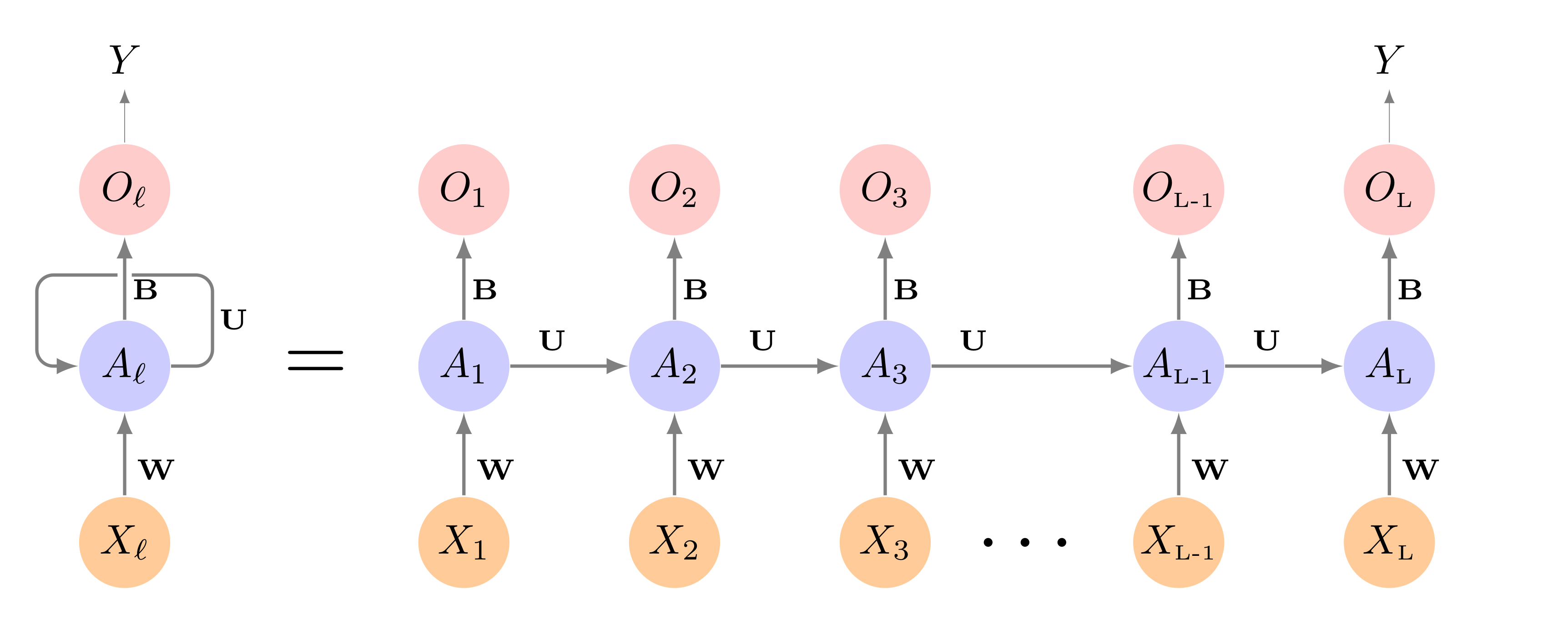
RNN
A recurrent neural network can be used to account the sequential order of the words.
Source: ISLR2
More Information
RNN
A recurrent neural network can be used to account the sequential order of each measurement.
Source: ISLR2
Neural Network
model <- nn_module(
  initialize = function(input_size = 10000 + 3) {
    self$dense1 <- nn_linear(input_size, 16)
    self$relu <- nn_relu()
    self$dense2 <- nn_linear(16, 16)
    self$output <- nn_linear(16, 1)
  },
  forward = function(x) {
    x |>
      self$dense1() |>
      self$relu() |>
      self$dense2() |>
      self$relu() |>
      self$output() |>
      torch_flatten(start_dim = 1)
  }
)fitted <- model |>
fit(
# we transform the training and validation data into torch tensors
list(
torch_tensor(as.matrix(x_train_1h[itrain,]), dtype = torch_float()),
torch_tensor(unlist(train$y[itrain]))
),
valid_data = list(
torch_tensor(as.matrix(x_train_1h[ival, ]), dtype = torch_float()),
torch_tensor(unlist(train$y[ival]))
),
dataloader_options = list(batch_size = 512),
epochs = 5
)
RNN Diagnostics

Neural Network
model <- nn_module(
  initialize = function() {
    self$rnn <- nn_rnn(3, 12, batch_first = TRUE)
    self$dense <- nn_linear(12, 1)
    self$dropout <- nn_dropout(0.2)
  },
  forward = function(x) {
    c(output, ...) %<-% (x |>
      self$rnn())
    output[,-1,] |>
      self$dropout() |>
      self$dense() |>
      torch_flatten(start_dim = 1)
  }
)