Main Types of Machine Learning
Supervised Learning
- Data includes inputs and outputs
- ML Models learns to map inputs → outputs
Unsupervised Learning
- Data has no labels
- Model discovers hidden patterns
with Torch
Machine Learning
Linear Regression
Neural Networks
Other Topics
Single-Layer Neural Network in R
Training/Validating/Testing Data
Machine Learning (ML) is the process of characterizing mathematical models, with the help of data, to predict outcomes of interest.
\[ Y = f(\boldsymbol X; \boldsymbol \theta) \]
Machine Learning
Linear Regression
Neural Networks
Other Topics
Single-Layer Neural Network in R
Training/Validating/Testing Data
Linear Regression is a tool to predict continuous random variables that are known to follow a Normal Distribution, with a set of known predictor variables.
Simple linear regression will model the association between one predictor variable and an outcome:
\[ \hat Y = \beta_0 + \beta_1 X \]
\(\beta_0\): Intercept term
\(\beta_1\): Slope term
Multivariable linear regression models are used when more than one explanatory variable is used to explain the outcome of interest.
To fit additional variable to the model, we will only need to add it to the model:
\[ \hat Y = \beta_0 +\beta_1 X_{1} + \beta_2 X_{2} \]
A categorical variable can be included in a model, but a reference category must be specified.
To fit a model with categorical variables, we must utilize dummy (binary) variables that indicate which category is being referenced. We use \(C-1\) dummy variables where \(C\) indicates the number of categories. When coded correctly, each category will be represented by a combination of dummy variables.
If we have 4 categories, we will need 3 dummy variables:
| Cat 1 | Cat 2 | Cat 3 | Cat 4 | |
|---|---|---|---|---|
| Dummy 1 | 1 | 0 | 0 | 0 |
| Dummy 2 | 0 | 1 | 0 | 0 |
| Dummy 3 | 0 | 0 | 1 | 0 |
Which one is the reference category?
Fitting an additional variable with 4 Categories
\[ \hat Y = \beta_0 +\beta_1 X_{1} + \beta_2 X_{2} + \beta_3 D_{1} + \beta_4 D_{2} + \beta_5 D_{3} \]
We find the values of \(\beta_0, \cdots, \beta_5\) that minimizes the following function for \(i\) data points:
\[ RSS = \sum^n_{i=1}(Y_i-\hat Y_i)^2 \]
\[ Y_i = \boldsymbol X_i^\mathrm T \boldsymbol \beta + \epsilon_i \]
\(Y_i\): Outcome Variable
\(\boldsymbol X_i\): Predictors
\(\boldsymbol \beta\): Coefficients
\(\epsilon_i\): error term
\[ \boldsymbol\beta = (\boldsymbol X^\mathrm T \boldsymbol X)^{-1} \boldsymbol X^\mathrm T \boldsymbol Y \]
Machine Learning
Linear Regression
Neural Networks
Other Topics
Single-Layer Neural Network in R
Training/Validating/Testing Data
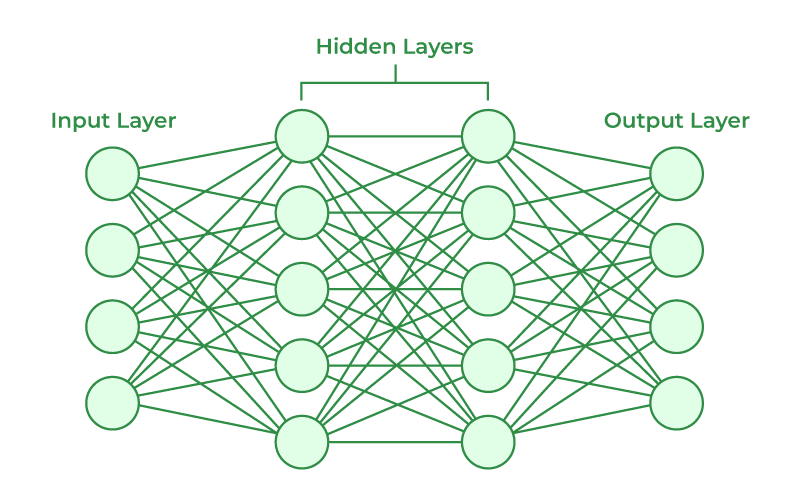
Neural networks are a type of machine learning algorithm that are designed to mimic the function of the human brain. They consist of interconnected nodes or “neurons” that process information and generate outputs based on the inputs they receive.
Neural networks are typically used for tasks such as image recognition, natural language processing, and prediction. They are capable of learning from data and improving their performance over time, which makes them well-suited for complex and dynamic problems.
\[ Y = f(\boldsymbol X; \boldsymbol \theta) \]
A single layer neural networks can be formulated as linear function:
\[ f(\boldsymbol X; \boldsymbol \theta) = \beta_0 + \sum^K_{k=1}\beta_kh_k(\boldsymbol X) \]
Where \(X\) is a vector of inputs of length \(p\) and \(K\) is the number of nodes (neurons), \(\beta_j\) are parameters
\[ h_k(\boldsymbol X) = g\left(\alpha_{k0} + \sum^p_{l=1}\alpha_{kl}X_{l}\right) \]
with \(g(\cdot)\) being a nonlinear activation function and \(\alpha_{kl}\) are the weights (parameters).
Fitting a neural network is the process of taking input data (\(X\)), finding the numerical values for the paramters that will minimize the following loss function, mean squared errors (MSE):
\[ \frac{1}{n}\sum^n_{i-1}\left\{Y_i-f(\boldsymbol X; \boldsymbol \theta)\right\}^2 \]
Machine Learning
Linear Regression
Neural Networks
Other Topics
Single-Layer Neural Network in R
Training/Validating/Testing Data
Activation functions are used to create a nonlinear affect within the neural network. Common activation functions are
Sigmoidal: \(g(z) = \frac{1}{1+e^{-z}}\) (nn_sigmoidal)
ReLU (rectified linear unit): \(g(z) = (z)_+ = zI(z\geq0)\) (nn_relu)
Hyperbolic Tangent: \(g(z) = \frac{\sinh(z)}{\cosh(z)} = \frac{\exp(z) - \exp(-z)} {\exp(z) + \exp(-z)}\) (nn_tanh)
Otherwise, the neural network is just an overparameterized linear model.
The optimizer is the mathematical algorithm used to find the numerical values for the parameters \(\beta_j\) and \(\alpha_{kl}\).
The most basic algorithm used in gradient descent.
Machine Learning
Linear Regression
Neural Networks
Other Topics
Single-Layer Neural Network in R
Training/Validating/Testing Data
Build a single-layer neural network that will predict body_mass with the remaining predictors. The hidden layer will contain 20 nodes, and the activation functions will be ReLU.
Creates the functions needed to describe the details of each network.
Machine Learning
Linear Regression
Neural Networks
Other Topics
Single-Layer Neural Network in R
Training/Validating/Testing Data
When creating a model, we are interested in determining how effective the model will be in predicting a new data point, ie not in our training data.
The error rate is a metric to determine how often will future data points be when using our model.
The problem is how can we get future data to validate our model?
The Training/Validating/Testing Data set is a way to take the original data set and split into 3 seperate data sets: training, validating, and testing.
This is data used to create the model.
This is data used to evaluate the data during it’s creation. It is evaluate at each Iteration (Epoch)
This is data used to test the final model and compute the error rate.
Training Error Rate is the error rate of the data used to create the model of interest. It describes how well the model predicts the data used to construct it.
Test Error Rate is the error rate of predicting a new data point using the current established model.
m408.inqs.info/lectures/3a