Neural Networks
Classification
R Packages
Data in Python
Penguins Data
#> Rows: 333
#> Columns: 8
#> $ species     <fct> Adelie, Adelie, Adelie, Adelie, Adelie, Adelie, Adelie, Ad…
#> $ island      <fct> Torgersen, Torgersen, Torgersen, Torgersen, Torgersen, Tor…
#> $ bill_len    <dbl> 39.1, 39.5, 40.3, 36.7, 39.3, 38.9, 39.2, 41.1, 38.6, 34.6…
#> $ bill_dep    <dbl> 18.7, 17.4, 18.0, 19.3, 20.6, 17.8, 19.6, 17.6, 21.2, 21.1…
#> $ flipper_len <int> 181, 186, 195, 193, 190, 181, 195, 182, 191, 198, 185, 195…
#> $ body_mass   <int> 3750, 3800, 3250, 3450, 3650, 3625, 4675, 3200, 3800, 4400…
#> $ sex         <fct> male, female, female, female, male, female, male, female, …
#> $ year        <int> 2007, 2007, 2007, 2007, 2007, 2007, 2007, 2007, 2007, 2007…
Classification
Classification
Buliding Classifiers
Log-likelihood Function
Single-Layer Neural Network
Multi-Layer Neural Network
Generalizing Neural Networks
Classification
Classification in statistical learning terms indicates predicting a categorical random variable.
Example
Let’s say we are interested in predicting the penguin species: Gentoo, Chinstrap, and Adelie.
\[ Y = \left\{ \begin{array}{c} Gentoo \\ Chinstrap \\ Adelie \end{array} \right. \]
Common Methods
Naive Bayes Classifier
Tree-based Methods
Support Vector Machines
Logistic/Multinomial regression
Discriminant Analysis
We are primarily going to use a logistic model approach.
Model
\[ Y = f(\boldsymbol X; \boldsymbol \theta) \]
- \(\boldsymbol X\): a vector of predictor variables
- \(\boldsymbol \theta\): a vector of parameters
How do we model an outcome which is categorical, not a number?
Modeling Probabilities
To model categorical data, we will model the probability of oberving each specific category.
Neural Netork
Let
\[ \bmcH(\bX; \btheta_G) \]
\[ \bmcH(\bX; \btheta_A) \]
\[ \bmcH(\bX; \btheta_C) \]
be three functions related to neural networks.
Unnormalized Probability
\[ \tilde P\left(Y = Gentoo\right) = exp\left\{\bmcH(\boldsymbol X; \boldsymbol \theta_G)\right\} \]
\[ \tilde P\left(Y = Adelie\right) = exp\left\{\bmcH(\boldsymbol X; \boldsymbol \theta_A)\right\} \]
\[ \tilde P\left(Y = Chinstrap\right) = exp\left\{\bmcH(\boldsymbol X; \boldsymbol \theta_C)\right\} \]
Normalized Probability (softmax)
\[ f_G(\bX) = P\left(Y = Gentoo\right) = \frac{exp\left\{\bmcH(\boldsymbol X; \boldsymbol \theta_G)\right\}}{exp\left\{\bmcH(\boldsymbol X; \boldsymbol \theta_G)\right\} + exp\left\{\bmcH(\boldsymbol X; \boldsymbol \theta_A)\right\} + exp\left\{\bmcH(\boldsymbol X; \boldsymbol \theta_C)\right\}} \]
\[ f_A(\bX) = P\left(Y = Adelie\right) = \frac{exp\left\{\bmcH(\boldsymbol X; \boldsymbol \theta_A)\right\}}{exp\left\{\bmcH(\boldsymbol X; \boldsymbol \theta_G)\right\} + exp\left\{\bmcH(\boldsymbol X; \boldsymbol \theta_A)\right\} + exp\left\{\bmcH(\boldsymbol X; \boldsymbol \theta_C)\right\}} \]
\[ f_C(\bX) = P\left(Y = Chinstrap\right) = \frac{exp\left\{\bmcH(\boldsymbol X; \boldsymbol \theta_C)\right\}}{exp\left\{\bmcH(\boldsymbol X; \boldsymbol \theta_G)\right\} + exp\left\{\bmcH(\boldsymbol X; \boldsymbol \theta_A)\right\} + exp\left\{\bmcH(\boldsymbol X; \boldsymbol \theta_C)\right\}} \]
For J Categories
\[ f_j(\bX) = P\left(Y = j\right) = \frac{exp\left\{\bmcH(\boldsymbol X; \boldsymbol \theta_j)\right\}}{\sum^J_{j=1}exp\left\{\bmcH(\boldsymbol X; \boldsymbol \theta_j)\right\}} \]
Buliding Classifiers
Classification
Buliding Classifiers
Log-likelihood Function
Single-Layer Neural Network
Multi-Layer Neural Network
Generalizing Neural Networks
Neural Networks
Neural Networks are capable of classifying data by fitting
Multilayer Neural Network
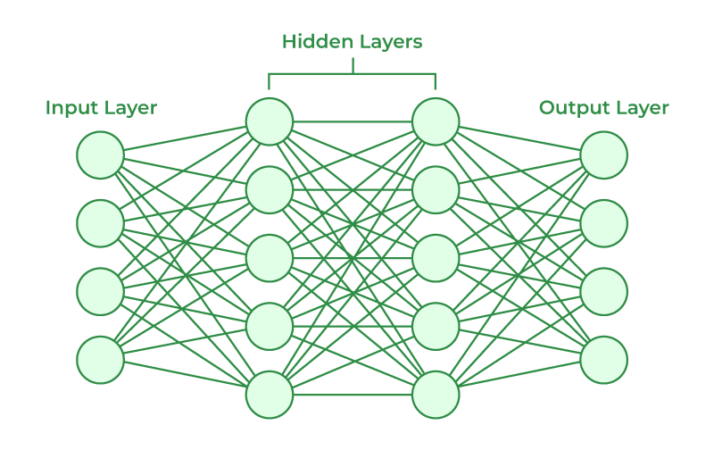
Hidden Layer 1
With \(p\) predictors of \(X\):
\[ h^{(1)}_k(X) = H^{(1)}_k = g\left\{\alpha_{k0} + \sum^p_{j=1}\alpha_{kj}X_{j}\right\} \] for \(k = 1, \cdots, K\) nodes.
Hidden Layer 2
\[ h^{(2)}_l(X) = H^{(2)}_l = g\left\{\beta_{l0} + \sum^K_{k=1}\beta_{lk}H^{(1)}_{k}\right\} \] for \(l = 1, \cdots, L\) nodes.
Hidden Layer 3 +
\[ h^{(3)}_m(X) = H^{(3)}_l = g\left\{\gamma_{m0} + \sum^L_{l=1}\gamma_{ml}H^{(2)}_{l}\right\} \] for \(m = 1, \cdots, M\) nodes.
Pre-Output Layer
\[ \bmcH(X) = \beta_{0} + \sum^M_{m=1}\beta_{m}H^{(3)}_m \]
Output Layer
\[ f_j(\bX) = P\left(Y = j\right) = \frac{exp\left\{\bmcH(\boldsymbol X; \boldsymbol \theta_j)\right\}}{\sum^k_{j=1}exp\left\{\bmcH(\boldsymbol X; \boldsymbol \theta_j)\right\}} \]
for all J functions (categories).
Log-likelihood Function
Classification
Buliding Classifiers
Log-likelihood Function
Single-Layer Neural Network
Multi-Layer Neural Network
Generalizing Neural Networks
Fitting Model
Fitting a neural network is the process of taking input data (\(X\)), finding the numerical values for the paramters that will maximizing (or in this case minimizing) the log-likelihood function, and finding the maximum likelihood estimator via gradient descent.
Log-likelihood Function
\[ \ell (\btheta) = - \sum^n_{i=1}\sum^k_{j=1} Y_{ij}\log\left\{f_j(\bX_i;\btheta)\right\} \]
\[ Y_{ij} = \left\{ \begin{array}{cc} 1 & j\mrth\ \mathrm{category} \\ 0 & \mathrm{otherwise} \end{array} \right. \]
Also known as cross-entropy.
Penguins Data
\[ \ell (\btheta) = - \sum^{333}_{i=1}\sum^3_{j=1} Y_{ij}\log\left\{f_j(\bX_i;\btheta)\right\} \]
Single-Layer Neural Network
Classification
Buliding Classifiers
Log-likelihood Function
Single-Layer Neural Network
Multi-Layer Neural Network
Generalizing Neural Networks
Single-Layer Neural Network
We will predict penguin species with a single-layer containing 10 nodes, and predict each species (3). We will use a ReLU activation function.
Penguin Data
Model Description
modelnn <- nn_module(
  initialize = function(input_size) {
    self$hidden1 <- nn_linear(in_features = input_size,
                              out_features = 10)
    self$output <- nn_linear(in_features = 10,
                             out_features = 3)

    self$activation <- nn_relu()
  },
  forward = function(x) {
    x |>
      self$hidden1() |>
      self$activation() |>
      self$output()
  }
)
Optimizer Set Up
Fit a Model
Multi-Layer Neural Network
Classification
Buliding Classifiers
Log-likelihood Function
Single-Layer Neural Network
Multi-Layer Neural Network
Generalizing Neural Networks
Multi-Layer Neural Network
Build a multi-layer neural network that will predict species with the remaining predictors and the following components:
- 3 Hidden Layers
- 20 nodes
- 10 nodes
- 5 nodes
- output is 3 seperate functions
- Use ReLU activation
Model Description
modelnn2 <- nn_module(
  initialize = function(input_size) {
    self$hidden1 <- nn_linear(in_features = input_size,
                              out_features = 20)
    self$hidden2 <- nn_linear(in_features = 20,
                              out_features = 10)
    self$hidden3 <- nn_linear(in_features = 10,
                              out_features = 5)

    self$output <- nn_linear(in_features = 5,
                             out_features = 3)

    self$activation <- nn_relu()
  },
  forward = function(x) {
    x |>
      self$hidden1() |>
      self$activation() |>

      self$hidden2() |>
      self$activation() |>

      self$hidden3() |>
      self$activation() |>

      self$output()
  }
)
Optimizer Set Up
Fit a Model
Generalizing Neural Networks
Classification
Buliding Classifiers
Log-likelihood Function
Single-Layer Neural Network
Multi-Layer Neural Network
Generalizing Neural Networks
Overfitting
Overfitting is the concept where the model becomes to well in predicting the data. The fear is that the model can only predict the data it was trained on, and not any other data point. Therfore, it cannot be deployed.
Therefore, we deploy three method to generalize the model:
- Get more data.
- Dropout
- Regularization
- Early Stopping
More Data
One of the best ways to prevent over fitting is get more data that is representative.
This ensures that the model is more generalizable.
Dropout
Dropout is the process where we randomly makes nodes into zero. This ensures that connections do not get to dependent on a critical node. It will need to rely on the other nodes to get better as well.
Dropout
modelnn3 <- nn_module(
  initialize = function(input_size) {
    self$hidden1 <- nn_linear(in_features = input_size,
                              out_features = 20)
    self$hidden2 <- nn_linear(in_features = 20,
                              out_features = 10)
    self$hidden3 <- nn_linear(in_features = 10,
                              out_features = 5)

    self$output <- nn_linear(in_features = 5,
                             out_features = 3)

    self$activation <- nn_relu()
    self$drop20 <- nn_dropout(p = 0.2)
    self$drop30 <- nn_dropout(p = 0.3)

  },
  forward = function(x) {
    x |>
      self$hidden1() |>
      self$activation() |>
      self$drop20() |>

      self$hidden2() |>
      self$activation() |>
      self$drop30() |>

      self$hidden3() |>
      self$activation() |>

      self$output()
  }
)Regularization
Regularization is the process where we add a penalty term to all the parameters and when fitting the data. This will ensure that the certain parameters will go to zero.
\[ \ell (\btheta) = - \sum^n_{i=1}\sum^k_{j=1} Y_{ij}\log\left\{f_j(\bX_i;\btheta)\right\} - \lambda \sum_r |\btheta_r| \]
Regularization
Early Stopping
We can reduce the number of epochs to train our model and so the parameters do not converge. This will allow the model to not fully explain the data, and in return, be more generalizable to new data.
Early Stopping
m408.inqs.info/lectures/5a