Linear Regression

Learning Objectives

• Associations

• Linear Regression

• Conducting it in R

Associations

Types of Associations

• Categorical vs Continuous

• Categorical vs Categorical

• Continuous vs Continuous

Categorical vs Continuous

Describing the relationship between categorical and continuous variables can be done by stratifying by the categorical variable and finding the mean or median, or conducting a statistical test:

• t-tests

• ANOVA

Measuring the association between species and flipper length from palmerpenguins:

# Stratification
penguins |>  drop_na()  |> 
  group_by(species) |>  
  summarise(mean = mean(flipper_length_mm),
            median = median(flipper_length_mm))

#> # A tibble: 3 × 3
#>   species    mean median
#>   <fct>     <dbl>  <dbl>
#> 1 Adelie     190.    190
#> 2 Chinstrap  196.    196
#> 3 Gentoo     217.    216

# ANOVA
species_aov <- aov(flipper_length_mm ~ species, penguins)
tidy(species_aov)

#> # A tibble: 2 × 6
#>   term         df  sumsq  meansq statistic    p.value
#>   <chr>     <dbl>  <dbl>   <dbl>     <dbl>      <dbl>
#> 1 species       2 52473. 26237.       595.  1.35e-111
#> 2 Residuals   339 14953.    44.1       NA  NA

Categorical vs Categorical

Comparing 2 categorical variables can be done by computing proportions or conducting a chi-square test. Below is an example comparing

# Count and Proportions
penguins |>  group_by(species, island) |> 
  summarise(count = n(), proportions = n() / nrow(penguins))

#> # A tibble: 5 × 4
#> # Groups:   species [3]
#>   species   island    count proportions
#>   <fct>     <fct>     <int>       <dbl>
#> 1 Adelie    Biscoe       44       0.128
#> 2 Adelie    Dream        56       0.163
#> 3 Adelie    Torgersen    52       0.151
#> 4 Chinstrap Dream        68       0.198
#> 5 Gentoo    Biscoe      124       0.360

# Chi-Square Test
penguins |> with(chisq.test(species, island))

#> 
#>  Pearson's Chi-squared test
#> 
#> data:  species and island
#> X-squared = 299.55, df = 4, p-value < 2.2e-16

Continuous vs Continuous

To understand the relationship between two continuous random variables, we can use the following:

• Correlation

• Linear Regression

Correlation

Correlations measures the association between 2 continuous random variables.

• Pearson’s Correlation

• Spearman’s Correlation

• Kendall’s Tau

# Pearson's Correlation
penguins |> drop_na() |> cor.test(~ body_mass_g + flipper_length_mm, 
                                  data = _)

#> 
#>  Pearson's product-moment correlation
#> 
#> data:  body_mass_g and flipper_length_mm
#> t = 32.562, df = 331, p-value < 2.2e-16
#> alternative hypothesis: true correlation is not equal to 0
#> 95 percent confidence interval:
#>  0.8447622 0.8963550
#> sample estimates:
#>       cor 
#> 0.8729789

# Spearman's Correlation 
penguins |>  drop_na() |> cor.test(~ body_mass_g + flipper_length_mm,
                                   data = _,
                                   method = "spearman")

#> 
#>  Spearman's rank correlation rho
#> 
#> data:  body_mass_g and flipper_length_mm
#> S = 982284, p-value < 2.2e-16
#> alternative hypothesis: true rho is not equal to 0
#> sample estimates:
#>       rho 
#> 0.8403902

# Kendall's Tau
penguins |>  drop_na() |> cor.test(~ body_mass_g + flipper_length_mm,
                                   data = _,
                                   method = "kendall")

#> 
#>  Kendall's rank correlation tau
#> 
#> data:  body_mass_g and flipper_length_mm
#> z = 17.683, p-value < 2.2e-16
#> alternative hypothesis: true tau is not equal to 0
#> sample estimates:
#>       tau 
#> 0.6614597

Scatter Plot

Linear Regression

Linear Regression

Linear regression is used to model the association between a set of predictor variables (x’s) and an outcome variable (y). Linear regression will fit a line that best describes the data points.

Scatter Plot

Simple Linear Regression

Simple linear regression will model the association between one predictor variable and an outcome:

\[ Y = \beta_0 + \beta_1 X + \epsilon \]

• \(\beta_0\): Intercept term

• \(\beta_1\): Slope term

• \(\epsilon\sim N(0,\sigma^2)\)

Estimated Model

\[ \hat Y = \hat \beta_0 + \hat \beta_1 X \]

Process

Process

Sums of Error Squared

\[ RSS = \sum^n_{i=1}(Y_i-\hat Y_i)^2 \]

Searching

Searching

Searching

Searching

Final

R Examples

R Formulas

In R, we create a formula using the tilde

Outcome Variable tilde Independent Variables

ooutcome_variable_name ~ independent_variable_name

R Example

Applying a linear regression model to body_mass_g (Predictor) and flipper_length_mm (Outcome) from penguins:

• R Output
• Scatter Plot

#> 
#> Call:
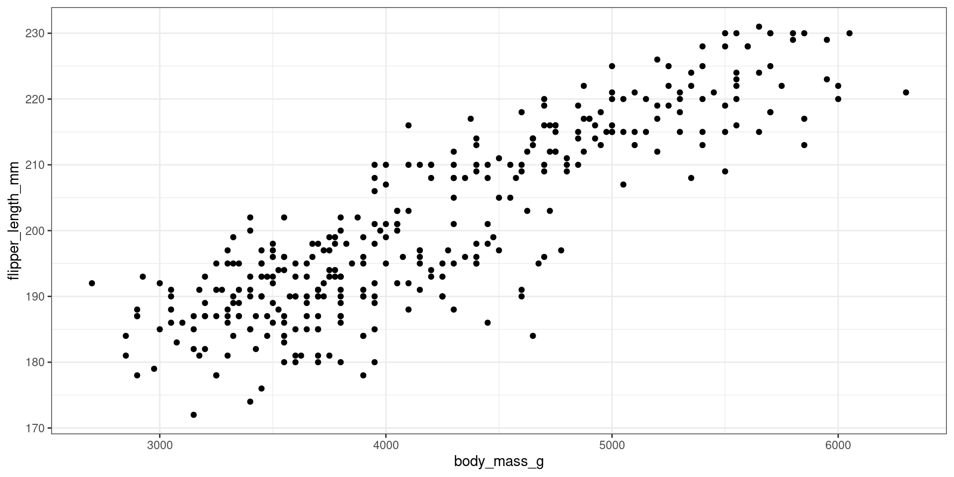
#> lm(formula = flipper_length_mm ~ body_mass_g, data = penguins)
#> 
#> Residuals:
#>      Min       1Q   Median       3Q      Max 
#> -23.7626  -4.9138   0.9891   5.1166  16.6392 
#> 
#> Coefficients:
#>              Estimate Std. Error t value Pr(>|t|)    
#> (Intercept) 1.367e+02  1.997e+00   68.47   <2e-16 ***
#> body_mass_g 1.528e-02  4.668e-04   32.72   <2e-16 ***
#> ---
#> Signif. codes:  0 '***' 0.001 '**' 0.01 '*' 0.05 '.' 0.1 ' ' 1
#> 
#> Residual standard error: 6.913 on 340 degrees of freedom
#>   (2 observations deleted due to missingness)
#> Multiple R-squared:  0.759,  Adjusted R-squared:  0.7583 
#> F-statistic:  1071 on 1 and 340 DF,  p-value: < 2.2e-16

Interpretation

\[ \hat y = 136.73 + 0.015 x \]

Simulation Example

Generate X Values

Simulate 250 independent values (x) from \(N(3, 1)\) and plot a histogram

x <- rnorm(250, 3, 1)

Generate Y Values

Create a new variable with the following formula:

\[ Y_i = 3 X_i + 20 \]

Create a Scatter Plot

Generate Error Term

Generate \(\epsilon_i\sim N(0, 2)\)

Create a histogram

Add error term

Create final form of \(Y_i\):

\[ Y_i = 3 X_i + 20 + \epsilon_i \]

Create a scatter plot

Simulation Study

To confirm that lm works, repeat the process 100 times and obtain the average \(\beta\) estimates:

1. Generate 250 X values
2. Create Y Value
3. Add error term
4. Fit Model
5. Store Values
6. Find the means of the coefficient

R Code of Simulation Study

## Original Code

x <- rnorm(250, 3, 1)
py <- 3 * x + 20
err <- rnorm(250, 0, 2)
y <- py + err
res <- lm(y ~ x)
coef(res)

#> (Intercept)           x 
#>    20.85743     2.73536

# Simulation Study
sim <- \(i){
  x <- rnorm(250, 3, 1)
  py <- 3 * x + 20
  err <- rnorm(250, 0, 2)
  y <- py + err
  res <- lm(y ~ x)
  return(coef(res))
}

sim_results <- sapply(1:1000, sim)
rowMeans(sim_results)

#> (Intercept)           x 
#>   20.018763    2.994175