Convolutional
Neural Networks
Model Building
R Packages
Python Data
import torch
import torchvision
import torchvision.transforms as transforms

transform = transforms.Compose(
    [transforms.ToTensor(),
     transforms.Normalize((0.5, 0.5, 0.5), (0.5, 0.5, 0.5))])

batch_size = 4

trainset = torchvision.datasets.CIFAR10(root='./data', train=True,
                                        download=True, transform=transform)
trainloader = torch.utils.data.DataLoader(trainset, batch_size=batch_size,
                                          shuffle=True, num_workers=2)

testset = torchvision.datasets.CIFAR10(root='./data', train=False,
                                       download=True, transform=transform)
testloader = torch.utils.data.DataLoader(testset, batch_size=batch_size,
                                         shuffle=False, num_workers=2)

classes = ('plane', 'car', 'bird', 'cat',
           'deer', 'dog', 'frog', 'horse', 'ship', 'truck')
Loading Data
Loading Data
Building CNNs
Speed Up Training
Transfer Learning
Loading Data
Building CNNs
Loading Data
Building CNNs
Speed Up Training
Transfer Learning
CNN Architecture

Convolutional Block 1
- Given an 3 channels (3 matrix)
- Apply a \(k_1 \times k_1\) convolutional filter for each individual channel
- Add up the results for each channel by convolutional filter
- Apply a activation function
- Pool the data using a \(\varrho_1 \times \varrho_1\) window matrix
- Repeat the process for the remaining \(\varkappa_1\) filters
- The number of channels available as input
- The size of the convolutional filter (\(k_1\))
- The activation function
- The pooling mechanism
- Define the size of the window matrix (\(\varrho_h\))
- Define how many convolutional filters will be used (\(\varkappa_1\))
Convolutional Block 2+ (h=h)
- Use the number of channels from the previous block (\(\varkappa_{h-1}\))
- Apply a \(k_h \times k_h\) convolutional filter for each individual channel
- Add up the results for each channel by convolutional filter
- Apply a activation function
- Pool the data using a \(\varrho_h \times \varrho_h\) window matrix
- Repeat the process for the remaining \(\varkappa_h\) filters
- The number of channels available as input
- The size of the convolutional filter (\(k_h\))
- The activation function
- The pooling mechanism
- Define the size of the window matrix (\(\varrho_h\))
- Define how many convolutional filters will be used (\(\varkappa_h\))
Flattening
Once the images has been pooled to a select pixels or features. The images are flattened to a set of inputs.
These inputs are used to a traditional neural network to classify an image.
Hidden Layers
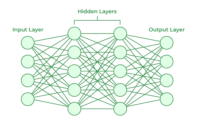
Neural Network
CIFAR Analysis
library(tidyverse)
library(torch)
library(luz)
library(torchvision)
set.seed(909)
torch_manual_seed(909)


# dir <- "./"
dir <- "../"


train_ds <- cifar10_dataset(
  # root = dir,
  train = TRUE,
  download = TRUE,
  transform = transform_to_tensor
)

test_ds <- cifar10_dataset(
  # dir,
  train = FALSE,
  download = TRUE,
  transform = transform_to_tensor
)

train_dl <- dataloader(train_ds,
  batch_size = 128,
  shuffle = TRUE
)

conv_block <- nn_module(
  initialize = function(in_channels, out_channels) {
    self$conv <- nn_conv2d(
      in_channels = in_channels,
      out_channels = out_channels,
      kernel_size = c(3,3),
      padding = "same"
    )
    self$relu <- nn_relu()
    self$pool <- nn_max_pool2d(kernel_size = c(2,2))
  },
  forward = function(x) {
    x |>
      self$conv() |>
      self$relu() |>
      self$pool()
  }
)

model <- nn_module(
  initialize = function() {
    self$conv <- nn_sequential(
      conv_block(3, 8),
      conv_block(8, 16)
    )
    self$output <- nn_sequential(
      nn_dropout(0.5),
      nn_linear(1024, 16),
      nn_relu(),
      nn_linear(16, 10)
    )
  },
  forward = function(x) {
    x |>
      self$conv() |>
      torch_flatten(start_dim = 2) |>
      self$output()
  }
)

first <- Sys.time()
fitted <- model |>
  setup(
    loss = nn_cross_entropy_loss(),
    optimizer = optim_rmsprop,

  ) |>
  set_opt_hparams(lr = 0.001) |>
  fit(
    train_dl,
    epochs = 3
  )
Sys.time() - first

plot(fitted)
Let’s Build Larger Models
Speed Up Training
Loading Data
Building CNNs
Speed Up Training
Transfer Learning
Speed Up Training
- GPU computing
- Batch Normalization
- Learning Rate
- Transfer Learning
Batch Normalization
Batch Normalization is the process where we scale the output of a convolutional block by the mean and standard deviation, which are parameters to be trained. This will allow the inputs for each layer to maintain the same units.
Adding Batch Normalization
We add nn_batch_norm2d() after each convolutional block.
Dynamic Learning Rate
Dynamic Learning Rate is the process where the neural network will changes the step size it will learn at each iteration. This will ensure that it will take large or smaller steps when it needs to.
Step Size
Small Step Sizes
It will get to the minimum at a snail space, but it will get there.
Large Step Sizes
It may skip the minimum at each time.
Learning Rate Finder
The idea is to choose a rate that ensure the loss function is being minimized.
Learning Rate Finder in R
We will use the lr_finder() to compute loss at different functions, and then plot them.
Learning Rate Scheduler
We will add the following code to fit() function:
Transfer Learning
Loading Data
Building CNNs
Speed Up Training
Transfer Learning
Transfer Learning
The idea of transfer learning models is to utilize pre-built models “knowledge” and transfer it to your own neural network that will be trained with your data.
Transfer Learning
- Download a pre-trained model.
- Identify the last layer of the model.
- Set all parameters (weights) not be trained.
- Replace the last layer of the model with your neural network needs.
- Train the model.
Transfer Learning
m408.inqs.info/lectures/7a