Recurrent
Neural Networks
R Packages
Python Data
Sequential Data
Sequential Data
Recurrent Neural Networks
Time Series
Predicting Electricity Demand
Sequential Data
Sequential data is data that is obtained in a series:
\[ X_{(0)}\rightarrow X_{(1)}\rightarrow X_{(2)}\rightarrow X_{(3)}\rightarrow \cdots\rightarrow X_{(J-1)}\rightarrow X_{(J)} \]
Stochastic Procceses
A stochastic process is a collection of random variables, that can be indexed by a parameters. Sequential data can be thought of as a stochastic process.
The generation of a variable \(X_{(j)}\) may or may not be dependent of the previous values.
Examples of Sequential Data
Documents and Books
Temperature
Stock Prices
Speech/Recordings
Handwriting
Recurrent Neural Networks
Sequential Data
Recurrent Neural Networks
Time Series
Predicting Electricity Demand
RNN
Recurrent Neural Networks are designed to analyze input data that is sequential data.
An RNN can accounts for the position of a data point in the sequence as well as the distance it has to other data points.
Using the data sequence, we can predict and outcome \(Y\).
RNN
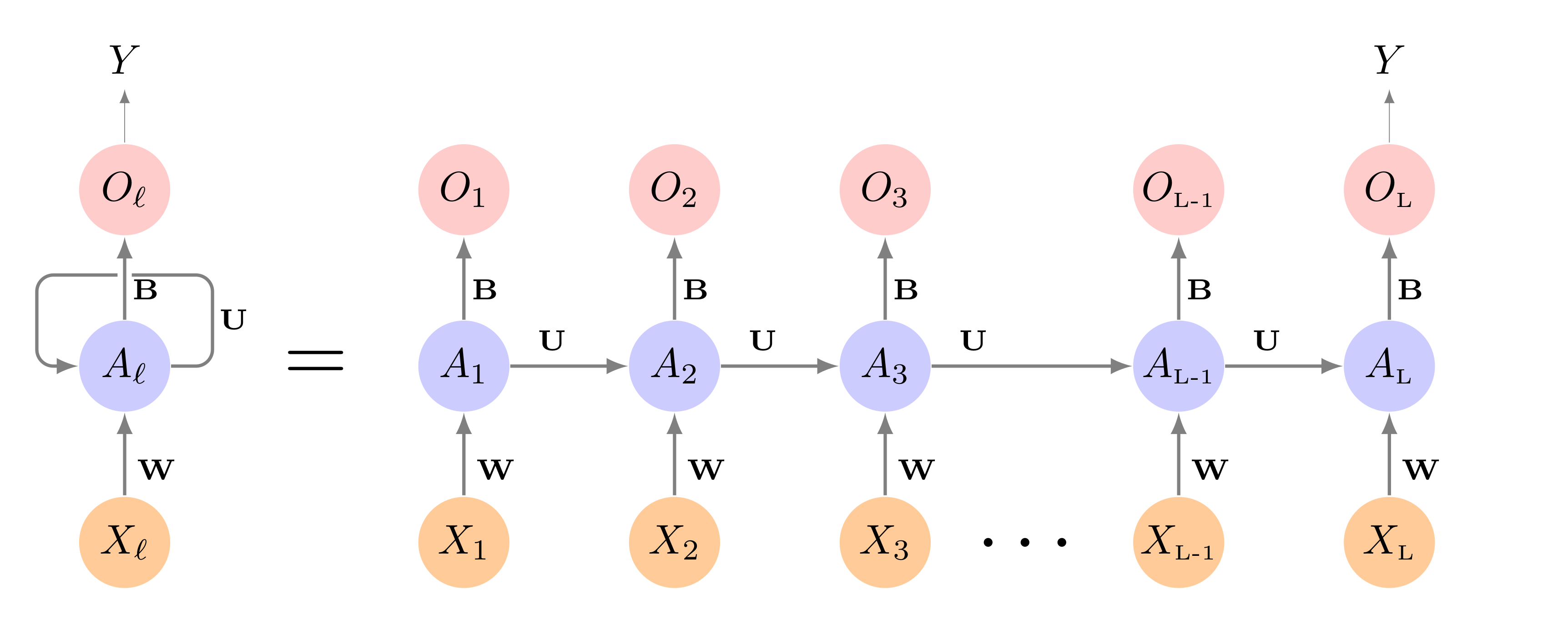
Source: ISLR2
RNN Neuron

RNN Neuron
RNN Inputs
\[ \boldsymbol X = (\boldsymbol x_0, \boldsymbol x_1, \boldsymbol x_2, \cdots, \boldsymbol x_{L-1}, \boldsymbol x_L) \]
where
\[ \boldsymbol x_{l} = (x_{l1},x_{l1}, \cdots, x_{lK}) \]
Hidden Layer
\[ A_{lj} = f(\sum_k\beta_{jk}\boldsymbol x_{lk} + \sum_m\bbeta_{jm}A_{(l-1)m} + \beta_{0j}) \]
- \(l\): Indexes the recurrent neuron
- \(j\): Indexes the node within the RNN neuron
- \(k\): Indexes the \(X\) input
- \(m\): Indexes the node of the previous RNN neuron
Output Layer
\[ O_{l} = g(\sum_j\gamma_{lj}A_{lj} + \gamma_{0l}) \]
Time Series
Sequential Data
Recurrent Neural Networks
Time Series
Predicting Electricity Demand
Time Series
A time series is a sequence of data points collected or recorded at successive, evenly spaced intervals of time. These data points can represent any variable that is observed or measured over time, such as temperature readings, stock prices, sales figures, or sensor data.
Data
\[ X_{(0)}\rightarrow X_{(1)}\rightarrow X_{(2)}\rightarrow X_{(3)}\rightarrow \cdots\rightarrow X_{(J-1)}\rightarrow X_{(J)} \]
RNN
A recurrent neural network can be used to account the sequential order of each measurement.
Source: ISLR2
Inputs and Outputs
- With Time-Series data, the data acts as both inputs and outputs.
- THere is a usually a lead-up in the input before we get an output.
Given the Data
\[ X_{(0)}\rightarrow X_{(1)}\rightarrow X_{(2)}\rightarrow X_{(3)}\rightarrow \cdots\rightarrow X_{(J-1)}\rightarrow X_{(J)} \]
Data Point 1
Input
\[ X_{(0)}, X_{(1)}, X_{(2)}, X_{(3)}, X_{(4)}, X_{(5)} \]
Output
\[ X_{(6)} \]
Data Point 2
Input
\[ X_{(1)}, X_{(2)}, X_{(3)}, X_{(4)}, X_{(5)}, X_{(6)} \]
Output
\[ X_{(7)} \]
Data Point 3
Input
\[ X_{(2)}, X_{(3)}, X_{(4)}, X_{(5)}, X_{(6)}, X_{(7)} \]
Output
\[ X_{(8)} \]
Data Point 4
Input
\[ X_{(3)}, X_{(4)}, X_{(5)}, X_{(6)}, X_{(7)}, X_{(8)} \]
Output
\[ X_{(9)} \]
Data Point 5
Input
\[ X_{(3)}, X_{(4)}, X_{(5)}, X_{(6)}, X_{(7)}, X_{(8)} \]
Output
\[ X_{(9)} \]
Time-Series Data Analysis
Most time-series data analysis is to understand cyclical trends and prediction.
More Information
Predicting Electricity Demand
Sequential Data
Recurrent Neural Networks
Time Series
Predicting Electricity Demand
Predicting Electricity Demand
We will use the vic_elec data set to be able to predict what the demand will be in a future time point.
Data Set
In order to fit a model with Torch, we need to provide a data set funcion that provides 2 values, a set of input and set of output. With Sequential data, values may be both outputs and inputs. We will use the dataset() to ensure that values can be used as both output and input.
RNN Neuron
Instead of the standard RNN Neuron, we will implement the Long Short-Term Memory Neuron.
Data Set
demand_dataset <- dataset(
  name = "demand_dataset",
  initialize = function(x, n_timesteps, sample_frac = 1) {
    self$n_timesteps <- n_timesteps
    self$x <- torch_tensor((x - train_mean) / train_sd)

    n <- length(self$x) - self$n_timesteps

    self$starts <- sort(sample.int(
      n = n,
      size = n * sample_frac
    ))
  },
  .getitem = function(i) {
    start <- self$starts[i]
    end <- start + self$n_timesteps - 1

    list(
      x = self$x[start:end],
      y = self$x[end + 1]
    )
  },
  .length = function() {
    length(self$starts)
  }
)
demand_hourly <- vic_elec |>
index_by(Hour = floor_date(Time, "hour")) |>
summarise(
Demand = sum(Demand))
demand_train <- demand_hourly |>
filter(year(Hour) == 2012) |>
as_tibble() |>
select(Demand) |>
as.matrix()
demand_valid <- demand_hourly |>
filter(year(Hour) == 2013) |>
as_tibble() |>
select(Demand) |>
as.matrix()
demand_test <- demand_hourly |>
filter(year(Hour) == 2014) |>
as_tibble() |>
select(Demand) |>
as.matrix()
train_mean <- mean(demand_train)
train_sd <- sd(demand_train)
n_timesteps <- 7 * 24Model
model <- nn_module(
  initialize = function(input_size,
                        hidden_size,
                        dropout = 0.2,
                        num_layers = 1,
                        rec_dropout = 0) {
    self$num_layers <- num_layers

    self$rnn <- nn_lstm(
      input_size = input_size,
      hidden_size = hidden_size,
      num_layers = num_layers,
      dropout = rec_dropout,
      batch_first = TRUE
    )

    self$dropout <- nn_dropout(dropout)
    self$output <- nn_linear(hidden_size, 1)
  },
  forward = function(x) {
    (x |>
      self$rnn())[[1]][, dim(x)[2], ] |>
      self$dropout() |>
      self$output()
  }
)
initialize = function(input_size,
hidden_size,
dropout = 0.2,
num_layers = 1,
rec_dropout = 0) {
self$num_layers <- num_layers
self$rnn <- nn_lstm(
input_size = input_size,
hidden_size = hidden_size,
num_layers = num_layers,
dropout = rec_dropout,
batch_first = TRUE
)
self$dropout <- nn_dropout(dropout)
self$output <- nn_linear(hidden_size, 1)
}Training
Predict and Visualize
demand_viz <- demand_hourly |>
  filter(year(Hour) == 2014, month(Hour) == 12)

demand_viz_matrix <- demand_viz |>
  as_tibble() |>
  select(Demand) |>
  as.matrix()

viz_ds <- demand_dataset(demand_viz_matrix, n_timesteps)
viz_dl <- viz_ds |> dataloader(batch_size = length(viz_ds))

preds <- predict(fitted, viz_dl)
preds <- preds$to(device = "cpu") |> as.matrix()
preds <- c(rep(NA, n_timesteps), preds)

pred_ts <- demand_viz |>
  add_column(forecast = preds * train_sd + train_mean) |>
  pivot_longer(-Hour) |>
  update_tsibble(key = name) |>
  as_tibble()

pred_ts |>
  ggplot(aes(Hour, value, color = name)) +
  geom_line() +
  scale_colour_manual(values = c("#08c5d1", "#00353f")) +
  theme_minimal() +
  theme(legend.position = "None")
m408.inqs.info/lectures/8a